14.1 Introduction

Analysing a set of rules with the aim to acquire useful knowledge about a new game is arguably the biggest, and most interesting, challenge for general game-playing systems. Most knowledge is only implicit in the description of a game and therefore needs to be learned, structured and verified before it can be used to improve play.

The range of game knowledge extends from basic properties, such as whether a game is zero-sum or cooperative, to expert knowledge that can fill entire databases, such as the world's chess knowledge accumulated over centuries of play.

The uses of knowledge in a general game player are equally wide. Simple properties can be used to decide on the right search method, like minimax with alpha-beta pruning in case a game has been identified as zero sum with alternating moves. Structural knowledge, e.g. of symmetries in a game, can be used to accelerate any search method. Knowledge of the value of different pieces or of different board regions can form the basis for evaluation functions, etcetera.

While the possibilities to acquire and use knowledge in a general game player are nearly limitless, in this and the following chapter we will consider a few approaches that are both relatively easy to implement and at the same time (almost) universally applicable.

We begin with a solution to a very basic problem that you need to solve if, for example, you want to transform a GDL description into a more efficient representation like a propositional network. To do so you need to determine the possible values for the arguments of each function and relation in a given game description. For some relations, like true, next, and does, this is easily computed from the base and action relation. But for auxiliary predicates and functions, their input values need to be explicitly computed.

14.2 Computing Domains

Computing the domains is actually fairly easy. We just need to examine the dependencies among the arguments and variables in each game rule. This can be achieved through the construction of the domain graph for a given GDL description.

The vertices of this graph include all function symbols and constants that occur in the rules. In our GDL-description for Tic-Tac-Toe in Chapter 2, for example, we find the following constants and functions, listed in the order of appearance.

white, black, mark, noop, 1, 2, 3, cell, x, o, b, control

The set of vertices also includes one node for each argument position of each predicate and function. An example are the two nodes row[1] and row[2] for the auxiliary binary function row from our Tic-Tac-Toe description.

The edges in the domain graph are directed. They indicate the dependencies between the constants, functions, and argument positions.

Definition 14.1 The domain graph for a set of GDL rules G is the smallest directed graph (V,E) with vertices V and edges E that satisfies all of the following.

1. c ∈ V for each constant c occurring in G.
2. p, p[1], …, p[n] ∈ V for each n-ary predicate or function symbol p occurring in G.
3. f → p[i] ∈ E for each occurrence of a function (or constant) f in the i-th argument of an expression p in the head of a rule in G.
4. p[j] → q[i] ∈ E whenever a variable X in a clause in G is shared by
   • the i-th argument of expression q in the head and
   • the j-th argument of expression p in the body.
5. E includes the three edges
   • base[1] → true[1]
   • input[1] → does[1]
   • input[2] → does[2]

As an example, recall one of the rules from our Tic-Tac-Toe description in chapter 2.

base(cell(M,N,x)) :- index(M) & index(N)

This rule gives rise to four edges in the Tic-Tac-Toe domain graph according to items 3 and 4 of Definition 14.1 as shown in the diagram below.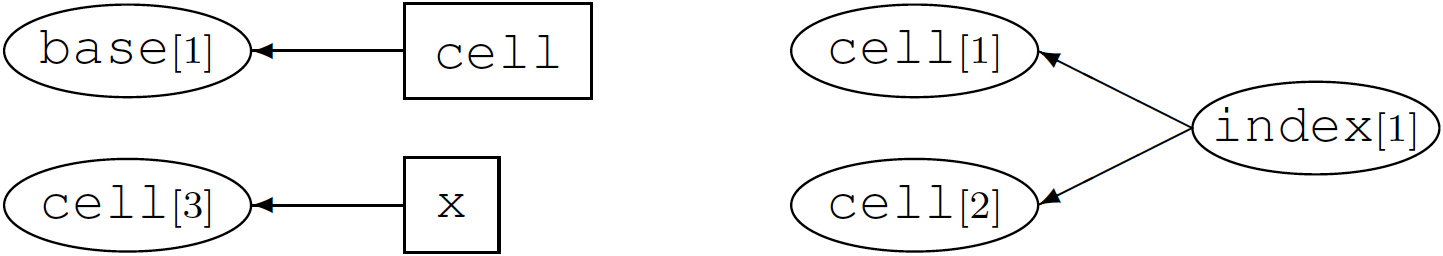

The edges cell → base[1] and x → cell[3] are obtained from the head of the clause. The edges connecting index[1] to cell[1] and cell[2] follow respectively from the shared variables M and N.

For another example, consider the clauses defining the auxiliary concepts of a row, column, diagonal, and line.

    line(X) :- row(M,X)
    line(X) :- column(N,X)
    line(X) :- diagonal(X)

    row(M,X) :-
      true(cell(M,1,X)) &
      true(cell(M,2,X)) &
      true(cell(M,3,X))

    column(N,X) :-
      true(cell(1,N,X)) &
      true(cell(2,N,X)) &
      true(cell(3,N,X))

    diagonal(X) :-
      true(cell(1,1,X)) &
      true(cell(2,2,X)) &
      true(cell(3,3,X)) &

    diagonal(X) :-
      true(cell(1,3,X)) &
      true(cell(2,2,X)) &
      true(cell(3,1,X)) &

Along with the base definition for cell,

    index(1)
    index(2)
    index(3)

    base(cell(M,N,x)) :- index(M) & index(N)
    base(cell(M,N,o)) :- index(M) & index(N)
    base(cell(M,N,b)) :- index(M) & index(N)

these rules determine edges in the Tic-Tac-Toe domain graph as follows.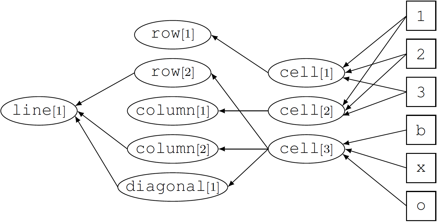

The domains for the four features can easily be computed from this graph by following backwards along all possible paths from the argument positions to the constants. The possible arguments of line, say, can be determined as follows.

Altogether we thus obtain the domains shown in the table below.

In the same way we can determine the domains for all other predicates and functions used in Chapter 2 to describe Tic-Tac-Toe.

14.3 Reducing the Domains Further

While the domain graph helps to identify the range of possible values for each individual argument, it does not consider dependencies between different argument positions of a predicate or function. As a consequence, it may still generate many unnecessary instances.

Take, for example, the following rules from a GDL description of the game of chess.

    coordinate(a)   coordinate(b)   coordinate(c)   coordinate(d)
    coordinate(e)   coordinate(f)   coordinate(g)   coordinate(h)

    coordinate(1)   coordinate(2)   coordinate(3)   coordinate(4)
    coordinate(5)   coordinate(6)   coordinate(7)   coordinate(8)

    next_file(a,b)  next_file(b,c)  next_file(c,d)  next_file(d,e)
    next_file(e,f)  next_file(f,g)  next_file(g,h)

    next_rank(1,2)  next_rank(2,3)  next_rank(3,4)  next_rank(4,5)
    next_rank(5,6)  next_rank(6,7)  next_rank(7,8)

    adjacent(X1,X2) :-
       next_file(X1,X2)
    adjacent(X1,X2) :-
       next_file(X2,X1)
    adjacent(Y1,Y2) :-
       next_rank(Y1,Y2)
    adjacent(Y1,Y2) :-
       next_rank(Y2,Y1)

    kingmove(U,V,U,Y) :-
       adjacent(V,Y) & coordinate(U)
    kingmove(U,V,X,V) :-
       adjacent(U,X) & coordinate(V)
    kingmove(U,V,X,Y) :-
       adjacent(U,X) & adjacent(V,Y)

The rules define a king's move as going one square in either direction, that is, vertically, horizontally, or diagonally. From the domain graph we can compute the possible values for the arguments of the five predicates as shown below.

But many of the instances thus obtained are unnecessary because they will never be referred to when playing the game.

To begin with, the domains for both adjacent(X,Y) and kingmove(U,V,X,Y) do not distinguish between file and rank coordinates. As a consequence, the domain graph generates superfluous instances like for example adjacent(a,2) or kingmove(d,e,5,6).

Even among the instances of kingmove(U,V,X,Y) for which both (U,V) and (X,Y) are proper squares, the vast majority is not needed given the limited mobility of a king: For every (U,V) there is a maximum of eight squares (X,Y) that a king can reach in one move. If we were able to identify all combinations of arguments that do not correspond to a possible move, such as kingmove(e,2,g,7), then this would significantly reduce the number of instances that we need to compute. A simple calculation shows how much can thus be saved. There are 16⁴ = 65,536 instances of kingmove with the domain as given in Table 14.2. If we respect the distinction between file and rank coordinates, this number reduces to 8⁴ = 4,096. Of these, less than 8²⋅ 8 = 512 correspond to an actual king move. (The exact number is 444 because a king at the border can reach no more than five squares and only three from a corner.)

The following procedure allows you to eliminate in a given game description G most of the instances of predicates that will never be derivable.

1. Build the domain graph for G to determine the maximal range of values for all predicates and functions in the game description.

2. Let G⁺ be obtained from G by

   • adding all facts true(t) and does(t₁,t₂) that follow from the domain graph; and
   • deleting all negative conditions from the rules in G.

3. For all possible predicate instances (except for the keywords true and does) with the domains obtained in step 1, check if they can actually be computed from G⁺. Keep only those that can.

4. For all possible instances of true(t) that follow from the domain graph, keep only those for which init(t) or next(t) can be computed from G⁺.

5. For all possible instances of does(t₁,t₂) that follow from the domain graph, keep only those for which legal(t₁,t₂) can be computed from G⁺.

Let's see how steps 1-3 of this process will indeed eliminate all unnecessary combinations of values from Table 14.2. To begin with, out of the 49 possible instances of next_file(X,Y) only the seven that are given as facts can be computed from the given game rules. The same is true for next_rank(X,Y). For adjacent(X,Y), we can compute 28 instances (out of a total of 16⋅16 = 256), which rules out instances like, say, adjacent(a,2) and adjacent(8,2). Finally, the only computable instances of kingmove(U,V,X,Y) are those 444 that correspond to actual moves by a king.

The reason for augmenting G in step 2 by all possible state propositions and all actions is that many predicates directly or indirectly depend on them. An example from Tic-Tac-Toe is shown below.

    line(X) :- row(M,X)

    row(M,X) :-
      true(cell(M,1,X)) &
      true(cell(M,2,X)) &
      true(cell(M,3,X))

With all possible instances of true(cell(M,N,X)) in Tic-Tac-Toe added, it follows that each of the nine combinations of arguments for row(M,X) according to Table 14.1 may indeed at some point be true. The same holds for the three instances of line(X).

The reason for deleting all negative conditions in step 2 is that it would be incorrect to uphold them after having added all possible state propositions and actions. This can be seen, for example, with the rules for a draw in Tic-Tac-Toe.

    goal(white,50) :- ~line(x) & ~line(o)
    goal(black,50) :- ~line(x) & ~line(o)

Step 4 is used to identify propositions that can never be true in a reachable game state. Similarly, step 5 is used to identify actions that will never be possible in a reachable state. As an example, consider a further rule from the GDL description of chess, where the general concept of a king move from above is used to define the conditions under which a player can legally move his king.

    piece_owner_type(wk,white,king)
    piece_owner_type(bk,black,king)

    legal(P,move(K,U,V,X,Y)) :-
      true(control(P)) &
      piece_owner_type(K,P,king) &
      true(cell(U,V,K)) &
      kingmove(U,V,X,Y) &
      occupied_by_opponent_or_blank(X,Y,P) &
      ~threatened(P,X,Y)

Recall that we were able in step 3 to restrict the possible instances of kingmove(U,V,X,Y) to those for which (X,Y) is one square away from (U,V). The very same restriction follows for legal(white,move(wk,U,V,X,Y)) and legal(black,move(bk,U,V,X,Y)) according to the rule just given. Hence, step 5 eliminates all instances of moves of the form does(white,move(wk,U,V,X,Y)) and does(black,move(bk,U,V,X,Y)) for which the two squares are not adjacent.

If steps 4 and 5 lead to a reduction in the set of state propositions and actions, then step 3 can be repeated with this reduced set in order to possibly further constrain the derivable predicate instances. This, in turn, may lead to more reductions in steps 4 and 5, so that the whole process can be iterated until no more ground predicates, state propositions, or moves are eliminated.

14.4 Instantiating Rules

During the instantiation process, you can evaluate each condition of the form distinct(X,Y) in the body of a rule as soon as both arguments have received a value. If true, the condition itself can be removed, and if false, the entire instance of the rule should be deleted.

As an illustrative example, let's look at the Tic-Tac-Toe rule shown below.

    next(cell(M,N,b)) :-
      does(W,mark(J,K)) &
      true(cell(M,N,b)) &
      distinct(M,J)

From the domain computation we know that M,N,J,K ∈ {1,2,3} and W ∈ {x,o}. Hence, we can instantiate the rule in 3⁴⋅2 = 162 different ways. But every third of these instances violates the condition distinct(M,J), so that in fact only 108 need to be generated.

A fully instantiated game description can be reduced further in size by identifying supporting concepts that are being computed but never used as input by any of the game rules. Such instances can safely be removed together with their defining clauses. Again, this is a process that can be repeated until no further reduction is possible.

A point in case are the Tic-Tac-Toe rules defining a line.

    line(X) :- row(M,X)
    line(X) :- column(N,X)
    line(X) :- diagonal(X)

    row(M,X) :-
      true(cell(M,1,X)) &
      true(cell(M,2,X)) &
      true(cell(M,3,X))
      
    column(N,X) :-
      true(cell(1,N,X)) &
      true(cell(2,N,X)) &
      true(cell(3,N,X))

    diagonal(X) :-
      true(cell(1,1,X)) &
      true(cell(2,2,X)) &
      true(cell(3,3,X))

    diagonal(X) :-
      true(cell(1,3,X)) &
      true(cell(2,2,X)) &
      true(cell(3,1,X))

From Table 14.1 we know that X ∈ {b,x,o} for line(X). Indeed, line(b) is derivable in many reachable states, including the initial one. But the supporting concept of a line is needed only for the goal rules shown below, which do not refer to blank lines.

    goal(white,100) :- line(x) & ~line(o)
    goal(white,50) :- ~line(x) & ~line(o)
    goal(white,0) :- ~line(x) & line(o)

    goal(black,100) :- ~line(x) & line(o)
    goal(black,50) :- ~line(x) & ~line(o)
    goal(black,0) :- line(x) & ~line(o)

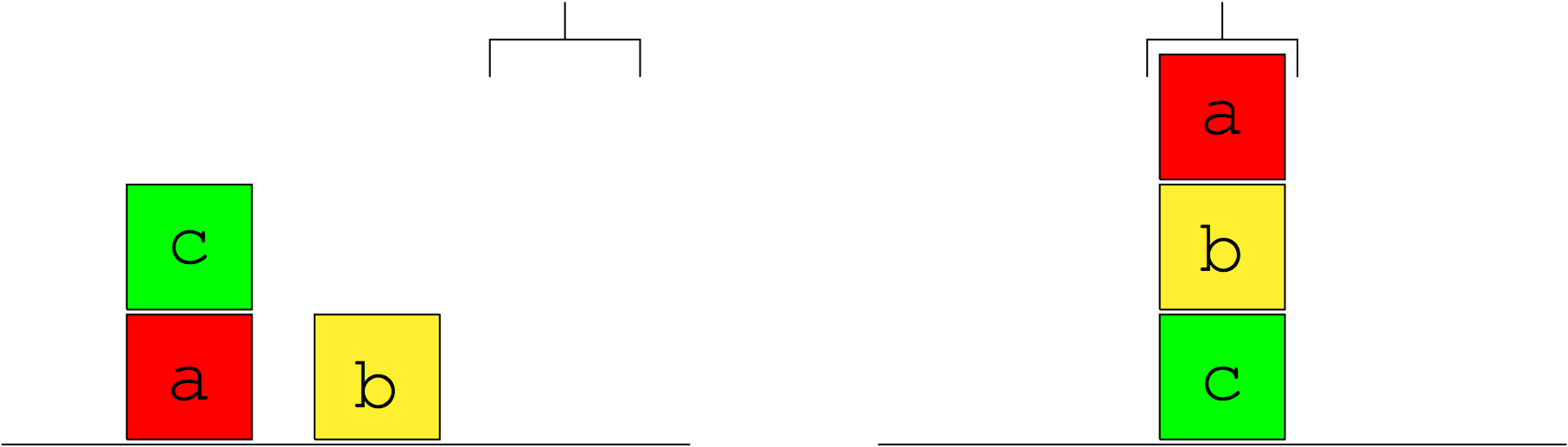
Consequently, we can delete each rule for line(X) that has been instantiated with X=b. This eliminates 7 of the 21 clauses with predicate line in the head obtained from the domains of Table 14.1. Moreover, once these have been removed there are no rules that use any of the conditions row(1,b), row(2,b), row(3,b), column(1,b), column(2,b), column(3,b) or diagonal(b). Hence, these and their defining clauses can be eliminated too.

The process of instantiating logic program rules is also known as grounding. Some of the techniques we described and others have been implemented in efficient systems that are commonly referred to as grounders and are not specific to GDL. An example is the grounder Gringo.

14.5 Analyzing the Structure of GDL Rules

Analzying the structure of GDL clauses has the goal to better understand the meaning of a rule by abstracting from the syntax details. This can be useful for many purposes. For instance, it enables the comparison of different formalizations of essentially the same rule. A general game player may thus be able to recognize a known game that just comes in a new guise.

Focusing on the structure of GDL rules also allows a general game-playing system to recognize symmetries in arbitrary games. As an example, the figure below illustrates two standard symmetries on the Tic-Tac-Toe board that you will be able to identify with the help of the structural rule analysis described in this section.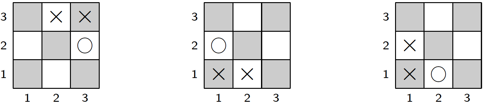

Determining symmetries like these requires to look at the game description as a whole and to see if some of its elements can be systematically exchanged with each other without affecting the meaning of any of the rules. The rules for winning or losing a game must be included in this analysis as symmetries can be broken by an asymmetric goal definition. If, say, a Tic-Tac-Toe player wins by filling a row but not a column with his or her markers, then the mirror symmetry in Figure 14.5 would no longer be applicable. (The 180° rotational symmetry, in contrast, would still apply.)

14.6 Rule Graphs

Much like the domain computation in section 14.2, the structural analysis can be performed on a graph constructed from the GDL rules. Specifically, the so-called rule graph for GDL game description is obtained through the four steps described below. Figures 14.6 - 14.8 illustrate this stepwise construction of the rule graph with a simple rule from our Tic-Tac-Toe description.

Prior to applying the following definition, all variables in a game description should be renamed so that no two rules share the same variables. Constants are treated like function symbols with zero arguments. The definition is rather involved, but an example immediately follows that illustrates in detail how to construct the graph step by step.

Definition 14.2 The rule graph for a set G of GDL rules is a colored directed graph (V,E,c) whose vertices V, edges E, and vertex coloring c are obtained as follows.

1. Add a vertex for each occurrence, in G, of a logical connective, predicate symbol, function symbol, and variable. Connect each vertex v that represents a logical connective, predicate, or function p with the vertices for the arguments of p.
2. For each vertex v thus obtained:
   • If v stands for an n-ary function or predicate symbol p that is not a GDL keyword,
     • add vertices labeled p[1], …, p[n];
     • for each such new vertex p[i], add a directed edge from p[i] to the vertex that in step 1 was created for the actual argument.
   • If v stands for the binary connective ":-" or a binary GDL keyword p, add a directed edge from the first to the second argument.
3. Add a vertex for each variable or symbol p that occurs in G and is not a GDL keyword. Add a directed edge from this vertex for p to
   • each occurrence node for p constructed in step 1, and
   • each node for p[1], …, p[n] constructed in step 2 if p is a function or predicate symbol with n arguments.
4. Color the vertices such that
   • each logical connective has a unique color;
   • each GDL keyword has a unique color; and
   • all other nodes are colored in one of six colors, which depends only on their type: predicate occurrence, function occurrence, variable occurrence, argument, variable symbol, or non-variable symbol.

For illustration, recall a simple rule from our Tic-Tac-Toe game description.

open :- true(cell(M,N,b))

The result of the first step in the construction of this clause's rule graph is shown below. Vertices are depicted in different shapes to indicate different types, which will help with the coloring in the end.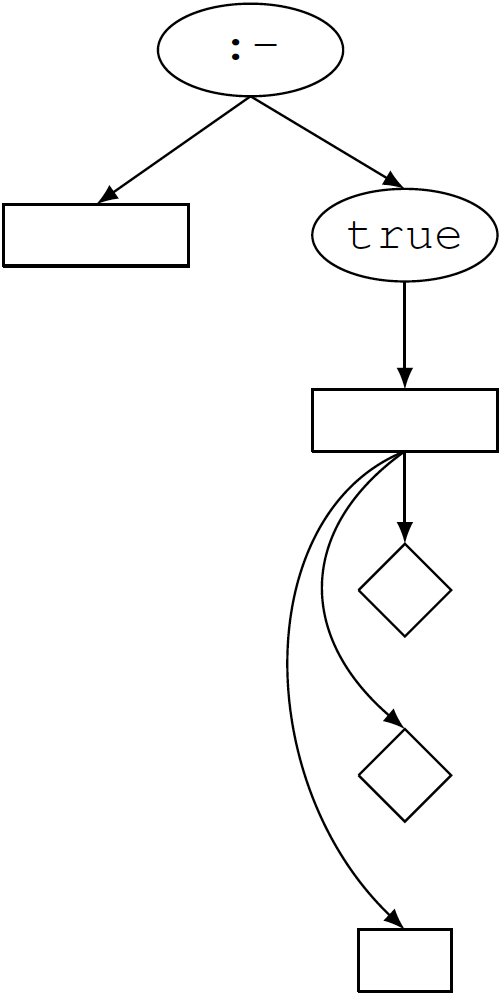

In the second step, argument position nodes are added for non-keyword cell and connected to the occurrences. Also added is an edge between the two arguments of the logical operator ":-".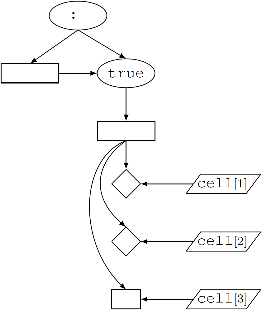

In step 3, nodes are added for each domain-dependent predicate symbol, function symbol, constant and variable itself.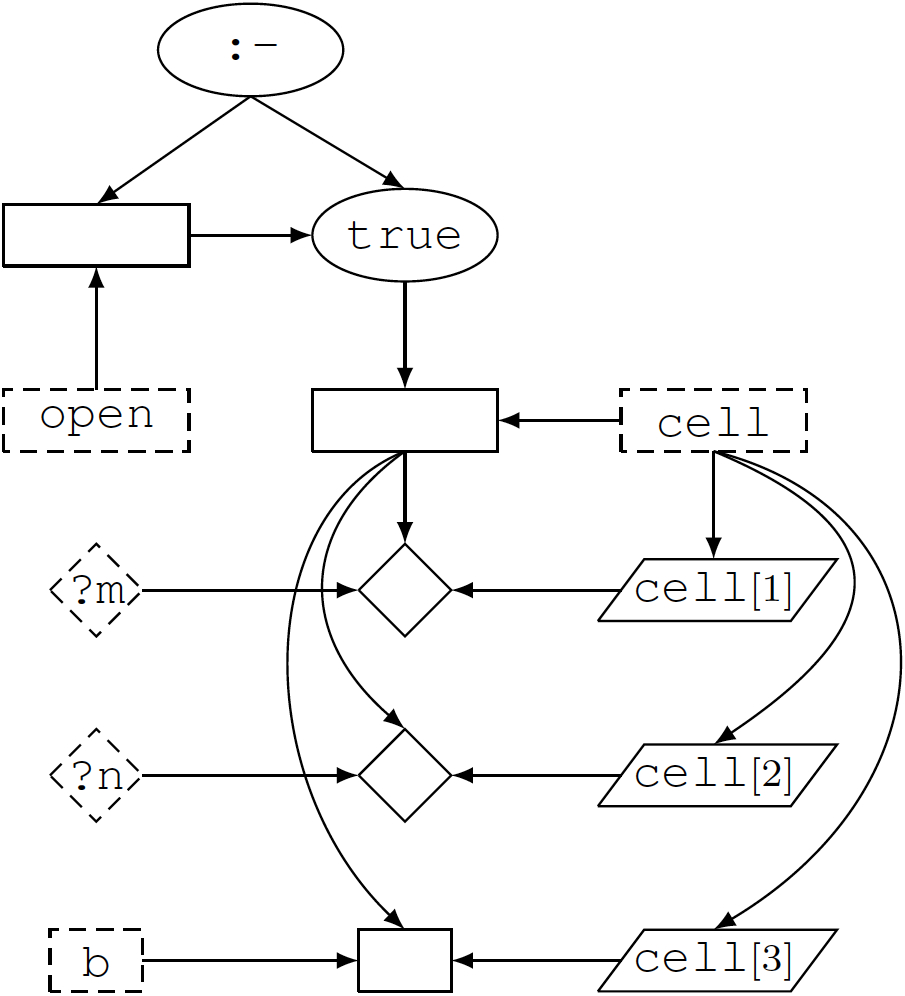

In step 4 all vertices get colored according to their type, which completes the construction of the rule graph. Since the structure of a set of rules is independent of the names given to the variables, functions and predicates, these symbols now become irrelevant. This will enable us to compare game axiomatizations that are structurally similar and differ only in the symbols being used.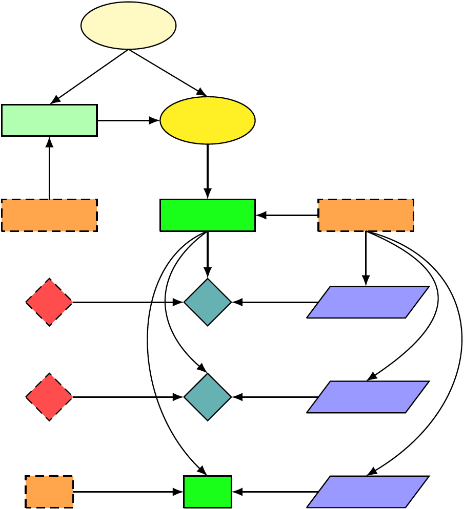

14.7 Using Rule Graphs

Determining the equivalence of game descriptions

The rule graph substitutes concrete symbols by abstract colors while maintaining the structure of the original rules. This allows to compare syntactically different but otherwise identical rules or game descriptions. An isomporhism between two colored graphs is a one-to-one mapping from the vertex set of one graph into the vertex set of the other that preserves both the edge structure and the coloring. Two graphs with an isomorphism between them are called isomorphic. Two GDL descriptions whose rule graphs are isomorphic describe essentially the same game.

As a simple example, the rule graph for our GDL description of Tic-Tac-Toe is isomorphic to the rule graph of any other description that just uses different coordinates, e.g. (a,a), (a,b), … instead of (1,1), (1,2), …, or different symbols for the two markers.

Computing symmetries

The rule graphs can moreover be used for symmetry detection. This requires to compute automorphisms, that is, on-to-one mappings from a rule graph into itself that are both structure- as well as color-preserving. As an example, consider exchanging two vertices the rule graph for Tic-Tac-Toe as follows.

This mapping constitutes an automorphism for the sub-graph depicted in Figure 14.10, which is obtained from the two GDL rules shown below.

init(cell(1,3,b))

init(cell(3,1,b))

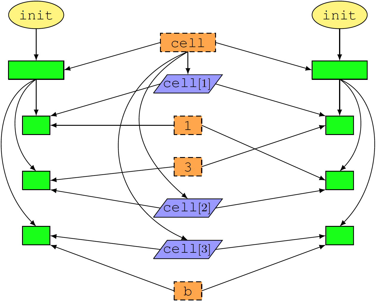
Our observation generalizes from this small sub-graph to the entire rule graph for our Tic-Tac-Toe description, which means that we have found a symmetry in this game. More specifically, we have discovered the 180° rotation symmetry from Figure 14.5 above, which is obtained by swapping the first and third coordinate, just like in our automorphism.

The mirror symmetry along the first diagonal of the Tic-Tac-Toe board is obtained by the following exchange of two vertices in the rule graph.

This mapping also can be shown to be an automorphism on the graphs depicted in Figures 14.9 and 14.10, respectively, and in fact provides an automorphism for the entire Tic-Tac-Toe rule graph.

The most common use of symmetry detection in general game players is to reduce the search space. You can, for example, prune a branch of a search tree when another branch with a symmetric joint move exists. You can also identify symmetric states and collate them in a single node in a search tree because, by definition, they must have the same value for all players.

Exercises

1. This exercise aims at determining the relevant ground instances of all rules of a single-player game called blocksworld.

   
   Figure 14.11 - A simple single-player game of moving toy blocks with a robot gripper. The goal is to transform the initial configuration on the left-hand side into the stack shown on the right-hand side.

   1. Let's start with the rules below.

         block(a)
         block(b)
         block(c)
         
         base(table(X)) :- block(X)
         base(clear(X)) :- block(X)
         base(on(X,Y)) :- block(X) & block(Y)
      

      From these rules draw the domain graph with nodes a,b,c,table,clear,on and block[1],base[1],table[1],clear[1],on[1],on[2].

   2. Now consider the next set of rules.

         succ(1,2)
         succ(2,3)
         succ(3,4)
         
         base(step(1))
         base(step(N)) :- succ(M,N)
      

      Extend the domain graph by the nodes 1,2,3,4,step along with nodes succ[1],succ[2],step[1] and add all edges that follow from the given clauses. Use the resulting graph to determine the possible arguments for keyword base.

   3. Extend the domain graph further according to the following rules.

         role(robot)
         
         input(robot,stack(X,Y))   :- block(X) & block(Y)
         input(robot,unstack(X,Y)) :- block(X) & block(Y)
      

      Use the resulting graph to determine the possible arguments for keyword input.

   4. Complete the domain graph using the remaining rules of the game shown below.

        init(table(a))
        init(table(b))
        init(on(c,a))
        init(clear(b))
        init(clear(c))
        init(step(1))
      
        legal(robot,stack(X,Y)) :-
          true(clear(X)) & true(clear(Y)) & distinct(X,Y)
        legal(robot,unstack(X,Y)) :-
          true(clear(X)) & true(on(X,Y))
      
        next(on(X,Y)) :- does(robot,stack(X,Y))
        next(on(X,Y)) :- does(robot,stack(U,V)) & true(on(X,Y))
        next(on(X,Y)) :-
          does(robot,stack(U,V)) & true(on(X,Y)) & distinct(U,X)
      
        next(table(X)) :- does(robot(unstack(X,Y))
        next(table(X)) :- does(robot(unstack(U,V)) & true(table(X))
        next(table(X)) :-
          does(robot(stack(U,V)) & true(table(X)) & distinct(U,X)
      
        next(clear(Y)) :- does(robot,unstack(X,Y))
        next(clear(Y)) :- does(robot,unstack(U,V)) & true(clear(Y))
        next(clear(Y)) :-
          does(robot,stack(U,V)) & true(clear(Y)) & distinct(V,Y)
      
        next(step(N)) :- true(step(M)) & succ(M,N)
      
        terminal :- true(step(4))
        terminal :- true(on(a,b)) & true(on(b,c))
      
        goal(robot,100) :- true(on(a,b)) & true(on(b,c))
        goal(robot,  0) :- ~true(on(a,b))
        goal(robot,  0) :- ~true(on(b,c))
      

      Use the resulting graph to determine the domain of next[1]. Which element from Domain(base[1]) is not a member of Domain(next[1])?

   5. Extend the given game description G to G⁺ by adding all facts true(t) and does(robot,t) that follow from the domain graph. Which of the instances of legal(robot,t) determined by the domain graph are not derivable from G⁺ and therefore can be removed?

   6. Use all of the above to determine only the relevant instances of the rule

      next(clear(Y)) :- does(robot,stack(U,V)) & true(clear(Y)) & distinct(V,Y)

      Hint: You should obtain just 6 out of the 27 instances that without further reductions would result from domain graph.

2. Implement the domain graph construction, the reduction strategy, and the grounding and try it out on the Tic-Tac-Toe game description and another standard GDL game of your choice.

3. This exercise is concerned with finding equivalences and symmetries in a variant of the Buttons and Lights game.

   1. Draw the rule graph for the following fact.

      role(player)

      Why would this graph be isomorphic to the rule graph for the clause "role(white)" but not for the clause "index(1)"?

   2. Draw the rule graph for the clause below.

      next(on(X)) :- ~true(on(X)) & does(player,toggle(X))

      Use the rule graph method to show that this clause is structurally equivalent to the rule

      next(p(Y)) :- does(white,q(Y)) & ~true(p(Y))

   3. Extend the graph for the entire game description given below.

          role(player)
          
          index(1)
          index(2)
          index(3)
          
          base(on(X)) :- index(X)
          input(player,toggle(X)) :- index(X)
          
          legal(player,toggle(X)) :- index(X)
          
          next(on(X)) :- ~true(on(X)) & does(player,toggle(X))
          next(on(X)) :- true(on(X)) & ~does(player,toggle(X))
          
          terminal :- true(on(1)) & true(on(2)) & true(on(3))
          goal(player,100) :- true(on(1)) & true(on(2)) & true(on(3))
      

      Use the rule graph method to find all symmetries in this game.

4. Implement the rule graph construction and try it out on the Tic-Tac-Toe game description and another standard GDL game of your choice. Search the web for a program to compute isomorphisms of graphs and use this to determine the symmetries in each of the two games.