1. Introduction

The most significant characteristic of General Game Playing is that players do not know the rules of games before those games begin. Game rules are communicated at runtime, and the players must be able to read and understand the descriptions they are given in order to play legally and effectively.

In General Game Playing, game rules are communicated to players in a formal language known as GDL (short for Game Description Language). GDL is an extension of a dynamic logic programming language called Epilog. (Epilog is an extension of pure Prolog that facilitates the representation of dynamic information.) There are just two significant differences between GDL and Epilog. (1) GDL includes a handful of reserved words that specialize it for the description of games. And (2) GDL has restrictions that assure that questions all game-related questions are decidable.

This article is an introduction to GDL and the issues that arise in using it to describe games. We start with an introduction to the modeling of games as dataset graphs. We then give a brief introduction to describing games as rules in GDL. We illustrate with the game description for Tic Tac Toe and then show how to simulate instances of the game using the game description.

2. Games as Dataset Graphs

Despite the variety of games treated in General Game Playing, all games share some common features. Each game takes place in an environment with finitely many states, with one distinguished initial state and one or more terminal states. In addition, each game has a fixed, finite number of players; each player has finitely many possible actions in any game state, and each state has an associated goal value for each player.

Given these features, we can think of a game as a state graph, like the one shown here. In this case, we have a game with one player, two actions (a and b), and eight states (named s₁, ... , s₈).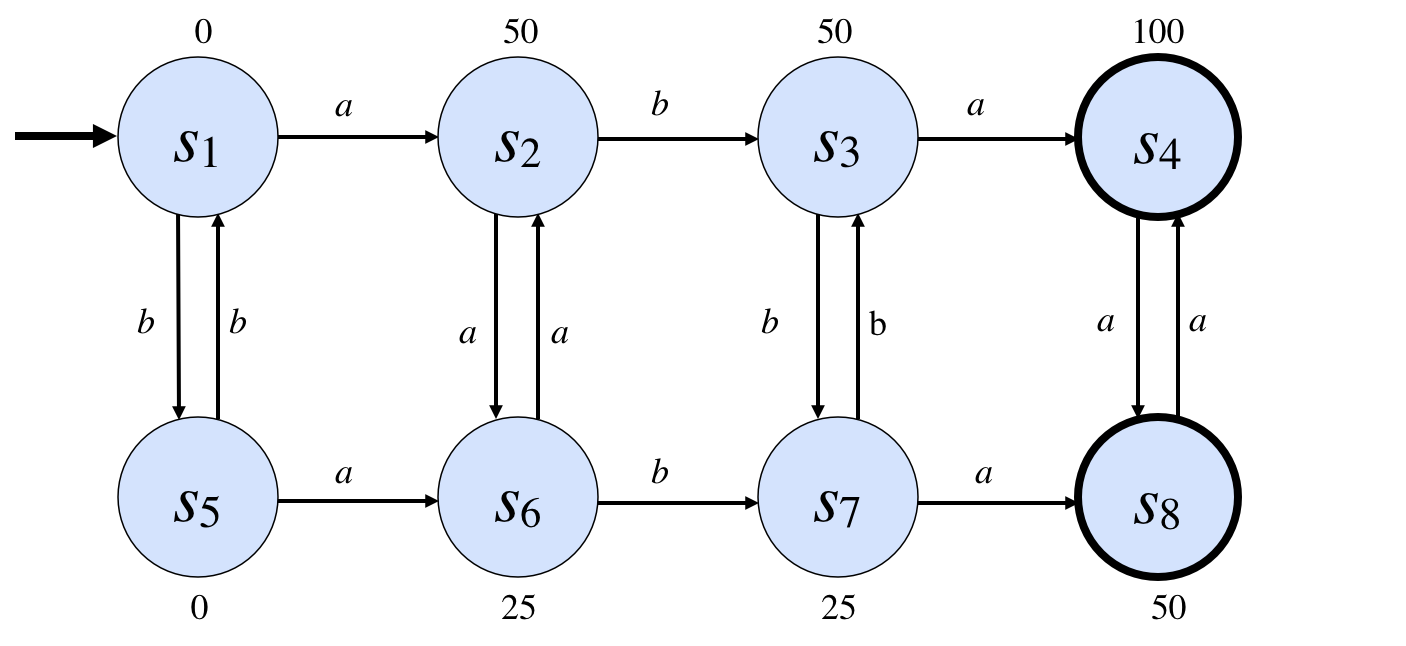

The arcs in this graph capture the transition function for the game. For example, if the game is in state s₁ and a player does action a, the game will move to state s₂. if the game is in state s₁ and a player does action b, the game will move to state s₅.

Each game has just one initial state, in this case s₁. However, there can be any number of terminal states, in this case s₄ and s₈.

The numbers associated with each state indicate the utilities of those states for the player. Players earn those scores only in terminal states. However, they are provided for all states and in some games indicate incremental progress.

We can extend this model to accommodate games with multiple players by making two modifications. (1) We annotate each state with rewards for all players in the game. (The rewards can be the same or different for different players.) (2) For each state, we specify which player is in control, i.e. whose turn it is to play. Turns need not strictly alternate; in some cases, a single player may get several turns in a row. (This model can be extended to games with simultaneous moves, but for the sake of simplicity, we avoid that complexity for now.)

This conceptualization of games is an alternative to the traditional extensive normal form definition of games as game trees. In a game tree, each node is linked to successors by arcs corresponding to the actions legal in the corresponding game state. While different nodes in game trees often correspond to different states, it is possible for different nodes to correspond to the same game state. (This happens when different sequences of actions lead to the same state.)

While extensive normal form is more appropriate for certain types of analysis, the state-based representation has advantages in General Game Playing. A state-based representation makes it possible to describe games more compactly; and, since game graphs are typically much smaller than game trees, it frequently decreases the computational cost of game analysis.

Since all of the games in General Game Playing are finite, it is possible, in principle, to linearize the corresponding state graph and use that linearization to communicate the game rules to players. Unfortunately, such explicit representations are not practical in all cases. Even though the numbers of states and actions are finite, these sets can be extremely large; and the corresponding graphs can be larger still. For example, in chess, there are more than 10⁴⁰ possible states.

In the vast majority of games, states and actions have composite structure that allows us to define a large number of states and actions in terms of a smaller number of more fundamental entities. In Chess, for example, states are not monolithic; they can be conceptualized in terms of pieces, squares, rows and columns and diagonals, and so forth.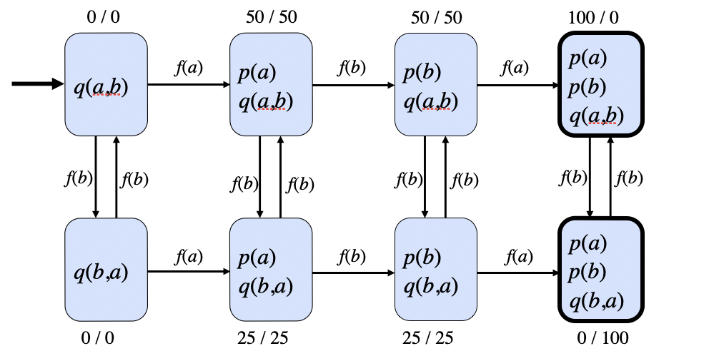

By exploiting this structure, it is possible to encode games in a form that is more compact than direct representation.

3. GDL

As just discussed, the states of games are modeled as sets of ground atomic propositions (datasets), and additional information is expressed in the form of rules that can be applied to these instances. View rules define higher level view relations in terms of lower level base relations (the relations used in datasets), and operation rules specify how the world state changes in response to the actions of the players.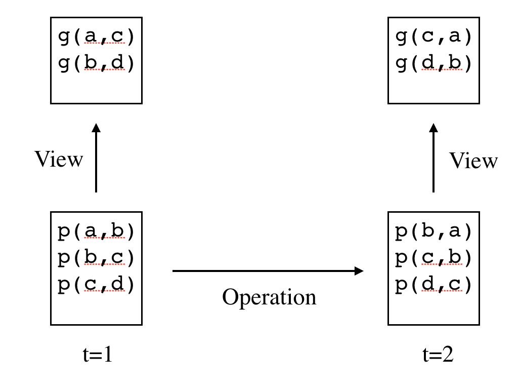

Views are defined by writing view rules. A view rule is an expression consisting of a distinguished atom, called the head, and zero or more literals, together called the body. The literals in the body are called subgoals. In what follows, we write rules as in the example shown below.

    g(X,Y) :- p(X,Y) & p(Y,Z)

Intuitively, a view rule is something like a reverse implication. For example, the rule above says that g is true of x and z if there is a y such that p is true of x and y and p is also true of y and z. (This is the view defined in the preceding figure.)

Operations are defined using operation rules. An operation rule is an expression of the form shown below. Each rule consists of (1) an action expression, (2) a double colon, (3) a literal or a conjunction of literals, (4) a double shafted forward arrow, and (5) a literal or an action expression or a conjunction of literals and action expressions. The action expression to the left of the double colon is called the head; the literals to the left of the arrow are called conditions; and the literals to its right are called effects.

    a :: p(X,Y) ==> ~p(X,Y) & p(Y,X)

This rule says that when the action a is performed, then, for any object y such that p holds of x and y, then p will be false of x and y in the next state and p will be true of y and x. (This is the operation defined in the preceding figure.)

In GDL, the meaning of some words in the language is fixed for all games (the game-independent vocabulary) while the meanings of all other words can change from one game to another (the game-specific vocabulary).

There are 101 game-independent object constants in GDL, viz. the base ten representations of the integers from 0 through 100, inclusive, i.e. 0, 1, 2, ... , 100. These are included for use as utility values for game states, with 0 being low and 100 being high. GDL has no game-independent function constants. However, there are eight game-independent relation constants, viz. the ones shown below.

role(a) means that a is a role in the game.

base(p) means that p is a base proposition in the game.

action(a) means that a is a feasible action in the game.

init(p) means that the proposition p is true in the initial state.

control(r) means that r is the player in control in the current state.

legal(a) means it is legal for the player in control to play action a in the current state.

goal(r,n) means that the current state has utility n for player r.

terminal means that the current state is a terminal state.

A game description in GDL is set of facts and rules defining these game-independent relations. (1) A GDL game description must give complete definitions for role, base, input, and init. (2) It must define legal and control and goal and terminal in terms of the game-specific base relations. (3) It must define the effects of each action. In the next section, we see how this is done in the context of one particular game, viz. Tic Tac Toe.

4. Tic Tac Toe

In Tic Tac Toe, we can think characterize states using two relations. The cell relation holds of a row and a column and a filler if and only if the cell in the specified row and column contains the specified filler. The filler can be the mark of either player or the symbol b (indicating that the cell is blank). The control relation holds of the player whose turn it is to play. The table below lists all of the possible propositions that can be formed using this conceptualization.

cell(1,1,x)
cell(1,2,x)
cell(1,3,x)
cell(2,1,x)
cell(2,2,x)
cell(2,3,x)
cell(3,1,x)
cell(3,2,x)
cell(3,3,x)

cell(1,1,o)
cell(1,2,o)
cell(1,3,o)
cell(2,1,o)
cell(2,2,o)
cell(2,3,o)
cell(3,1,o)
cell(3,2,o)
cell(3,3,o)

control(x)
control(o)

cell(1,1,b)
cell(1,2,b)
cell(1,3,b)
cell(2,1,b)
cell(2,2,b)
cell(2,3,b)
cell(3,1,b)
cell(3,2,b)
cell(3,3,b)

In Tic Tac Toe, there is only one type of action a player can perform - it can mark a cell. The binary operation mark together with a row m and a column n designates the action of placing a mark in row m and column n. The mark placed there depends on who does the action. The action base for this model is shown below.

mark(1,1)
mark(1,2)
mark(1,3)

mark(2,1)
mark(2,2)
mark(2,3)

mark(3,1)
mark(3,2)
mark(3,3)

The dataset shown below represents the initial state of Tic Tac Toe. All of the cells are blank and the x player is in control.

cell(1,1,b)
cell(1,2,b)
cell(1,3,b)
cell(2,1,b)
cell(2,2,b)
cell(2,3,b)
cell(3,1,b)
cell(3,2,b)
cell(3,3,b)
control(x)

Given the rules of Tic Tac Toe, all nine possible moves are legal in this state.

mark(1,1)
mark(1,2)
mark(1,3)
mark(2,1)
mark(2,2)
mark(2,3)
mark(3,1)
mark(3,2)
mark(3,3)

The game graph associated with this conceptualization consists of all feasible states with arcs for all legal actions. There are approximately 5040 states. Too big to draw here. And impractical as a way of communicating the game rules to the players. Luckily the description in GDL is much more compact.

We begin with an enumeration of roles. In this case, there are just two roles, here called x and o

    role(white)
    role(black)

We can characterize the propositions of the game as shown below.

    base(cell(M,N,x)) :- index(M) & index(N)
    base(cell(M,N,o)) :- index(M) & index(N)
    base(cell(M,N,b)) :- index(M) & index(N)

    base(control(white))
    base(control(black))

In GDL, symbols that begin with capital letters are variables, while symbols that begin with lower case letters are constants. The :- operator is read as "if" - the expression to its left is true if the expressions that follow it are true. See http://logicprogramming.stanford.edu for a full description of syntax and semantics of rules.

We can characterize the feasible actions for each role in similar fashion.

    action(mark(M,N)) :- index(M) & index(N)

    index(1)
    index(2)
    index(3)

Next, we characterize the initial state by writing all relevant propositions that are true in the initial state. In this case, all cells are blank; and the x player has control.

    init(cell(M,N,b)) :- index(M) & index(N)
    init(control(x))

With our declarations out of the way, we can get down to the dynamics of the game. First, we define legality. It is legal to mark a cell if that cell is blank.

    legal(mark(M,N)) :- cell(M,N,b)

Next, we look at the update rules for the game. The first rules says that, if w is the player in control, and w marks the cell in row m and column n, then that cell contains a w in the next state. The second rule says that the cell is no longer blank. The third and fourth rules describe the change of control that occurs when a player marks a cell.

    mark(M,N) :: control(W) ==> cell(M,N,W)
    mark(M,N) :: ~cell(M,N,b)
    mark(M,N) :: control(x) ==> ~control(x) & control(o)
    mark(M,N) :: control(o) ==> ~control(o) & control(x)

Goals. The x player gets a score of 100 if there is a line of x's and no line of o's. It gets 0 points if there is a line of o's and no line of x's. Otherwise, it gets 50 points. The rewards for the o player are analogous. The line relation is defined below.

    goal(x,100) :- line(x) & ~line(o)
    goal(x,50) :- ~line(x) & ~line(o)
    goal(x,0) :- ~line(x) &  line(o)

    goal(o,100) :- ~line(x) & line(o)
    goal(o,50) :- ~line(x) & ~line(o)
    goal(o,0) :- line(x) &  ~line(o)

Supporting concepts. A line is a row of marks of the same type or a column or a diagonal. A row of marks mean thats there three marks all with the same first coordinate. The column and diagonal relations are defined analogously.

    line(Z) :- row(M,Z)
    line(Z) :- column(M,Z)
    line(Z) :- diagonal(Z)

    row(M,Z) :- cell(M,1,Z) & cell(M,2,Z) & cell(M,3,Z)
    column(N,Z) :- cell(1,N,Z) & cell(2,N,Z) & cell(3,N,Z)
    diagonal(Z) :- cell(1,1,Z) & cell(2,2,Z) & cell(3,3,Z)
    diagonal(Z) :- cell(1,3,Z) & cell(2,2,Z) & cell(3,1,Z)

Termination. A game terminates whenever there is a line of marks of the same type or if the game is no longer open, i.e. there are no blank cells.

    terminal :- line(x)
    terminal :- line(o)
    terminal :- ~open

    open :- cell(M,N,b)

Note that, any of these relations can be assumed to be false if it is not provably true. Thus, we have complete definitions for the relations legal, goal, and terminal in terms of cell and control. The true relation starts out identical to init and on each step is changed to correspond to the extension of the next relation on that step.

Although GDL is designed for use in defining complete information games, it can be extended to partial information games. That said, the resulting descriptions are more verbose and more expensive to process.

5. Game Simulation Example

As an exercise in logic programming and GDL, let's look at the outputs of the ruleset defined in the preceding section at various points during an instance of the game.

To start, we can use the ruleset to compute the roles of the game. This is simple in the case of Tic-Tac-Toe, as they are contained explicitly in the ruleset.

    role(x)
    role(o)

We can also compute the relevant actions of the game. The extension of the action relation in this case consists of the nine sentences shown below.

    action(mark(1,1))
    action(mark(1,2))
    action(mark(1,3))
    action(mark(2,1))
    action(mark(2,2))
    action(mark(2,3))
    action(mark(3,1))
    action(mark(3,2))
    action(mark(3,3))

Similarly, we can compute the possible base propositions. Remember that this gives a list of all such propositions; only a subset will be true in any particular state.

    base(cell(1,1,x))    base(cell(1,1,o))    base(cell(1,1,b))
    base(cell(1,2,x))    base(cell(1,2,o))    base(cell(1,2,b))
    base(cell(1,3,x))    base(cell(1,3,o))    base(cell(1,3,b))
    base(cell(2,1,x))    base(cell(2,1,o))    base(cell(2,1,b))
    base(cell(2,2,x))    base(cell(2,2,o))    base(cell(2,2,b))
    base(cell(2,3,x))    base(cell(2,3,o))    base(cell(2,3,b))
    base(cell(3,1,x))    base(cell(3,1,o))    base(cell(3,1,b))
    base(cell(3,2,x))    base(cell(3,2,o))    base(cell(3,2,b))
    base(cell(3,3,x))    base(cell(3,3,o))    base(cell(3,3,b))
    base(control(x))
    base(control(o))

The first step in playing or simulating a game is to compute the initial state. We can do this by computing the init relation. As with roles, this is easy in this case, since the initial conditions are explicitly listed in the program.

    init(cell(1,1,b))
    init(cell(1,2,b))
    init(cell(1,3,b))
    init(cell(2,1,b))
    init(cell(2,2,b))
    init(cell(2,3,b))
    init(cell(3,1,b))
    init(cell(3,2,b))
    init(cell(3,3,b))
    init(control(x))

Once we have these conditions, we can turn them into a state description for the first step by asserting that each initial condition is true.

    cell(1,1,b)
    cell(1,2,b)
    cell(1,3,b)
    cell(2,1,b)
    cell(2,2,b)
    cell(2,3,b)
    cell(3,1,b)
    cell(3,2,b)
    cell(3,3,b)
    control(x)

Taking this input data and the logic program, we can check whether the state is terminal. In this case, it is not.

We can also compute the goal values of the state; but, since the state is non-terminal, there is not much point in doing that; but the description does give us the following values.

    goal(x,50)
    goal(o,50)

More interestingly, using this state description and the logic program, we can compute legal actions in this state. See below. The x player (the player in control) has nine possible actions (all marking actions).

    legal(mark(1,1))
    legal(mark(1,2))
    legal(mark(1,3))
    legal(mark(2,1))
    legal(mark(2,2))
    legal(mark(2,3))
    legal(mark(3,1))
    legal(mark(3,2))
    legal(mark(3,3))

Let's suppose that the x player chooses the first legal action.

    mark(1,1)

Now, combining this dataset with the state description above and the operation definitions, we can compute what must be true in the next state.

    cell(1,1,x)
    cell(1,2,b)
    cell(1,3,b)
    cell(2,1,b)
    cell(2,2,b)
    cell(2,3,b)
    cell(3,1,b)
    cell(3,2,b)
    cell(3,3,b)
    control(o)

This continues until we encounter a state that is terminal, at which point we can compute the goals of the players in a similar manner.